flowchart LR
    Record --> Data --> Tidy-data --> Data-analysis
Data wrangling
Data wrangling is the process of making data ready for modelling. It is a tedious task and involves different logical steps.
Core Concepts
Always look directly into data and see how it look like
Think how it should look like
Think how to rearrange Information to achieve what we want
Make sure that what we does is doing what we want at every step.
r is an excellent lower level language for data wrangling. The newer data.table make it even more faster and intuitive. data. table package in r is faster than not only tidyverse, it beats most other languages including python. Mainly used for data manipulation, it retains native data. frame and all functions written for base r and tidyverse work with data. table.
eg: % > % is called pipe function. It essentially means ‘take whatever on the left side and make it the first argument for anything on the right Side’. It comes with tidyverse package. It can also be used with data.table. 1
data.table
data.table looks like data.frame superficially but it is lot more efficient, fast and allow numerous actions by simple commands.
flowchart TD
A{data.table} --> B[i]
B --> C[subsetting row]
A --> D[j]
D --> E[subsetting & calculating in column]
A --> F[by]
F --> G[grouping]
A --> H[useful codes]
H --> I[fread]
H --> J[walrus]
Old data.frame allow sub-setting rows and selecting columns. data.table which uses the extended syntax
\[ dt[i,j,by] \]
allow lot more options.
i,j and by
iallows sub-setting and ordering row
dt[i] allow multiple actions at row level of the data. Fundamentally this can be grouped in to sub-setting and ordering.
flowchart TD
i --> subsetting
i --> ordering
Sub-setting
Let us take an example,
We have a data set called virtual.csv stored in our computer. The data belongs to a quasi experimental study which compared the effectiveness of virtual class room with respect to physical class room. It also compared the student perception of the two modalities on a likert scale. Study divided students in to two groups, virtual and physical and asked following questions:
- Is there any difference in the post test score of students in virtual and physical group?
- Is there any difference in the student perception in virtual and physical group about the modality of delivery of class?
We can bring it to r environment using fread command in the data.table library.
library(data.table)
dt=fread("virtual.csv")
Code
library(data.table)
dt=fread("virtual.csv")
We can see that it contains a set of simple data comparing the performance of medical students in physical classes vs virtual classes and their perceptions.
Select only virtual data
Assume, we want to see only the virtual class students. This can be easily achieved by sub-setting the type.class key in the data by “virtual” as shown below.
library(data.table)
dt=fread("virtual.csv")
dtv=dt[type.class == "virtual"]
head(dtv)
Code
library(data.table)
dt=fread("virtual.csv")
dtv=dt[type.class == "virtual"]
head(dtv)
##    idertifier type.class pretest.score pretest.rank posttest.score
##        <char>     <char>         <int>        <int>          <int>
## 1:       VIR1    virtual            40            2            100
## 2:       VIR2    virtual            40            2             95
## 3:       VIR3    virtual            60            3             85
## 4:       VIR4    virtual            40            2             70
## 5:       VIR5    virtual            60            3             75
## 6:       VIR6    virtual            60            3             90
##    posttest.rank   sex likert.1 likert.2 likert.3 likert.4 likert.5 likert.6
##            <int> <int>    <int>    <int>    <int>    <int>    <int>    <int>
## 1:             5     1        3        4        3        3        4        4
## 2:             5     1        3        5        4        2        3        4
## 3:             5     2        4        4        3        3        4        3
## 4:             4     2        5        4        4        2        3        4
## 5:             4     1        4        4        3        3        4        3
## 6:             5     1        3        5        3        2        3        4
##    likert.7 likert.8 likert.9 likert.10 likert.total
##       <int>    <int>    <int>     <int>        <num>
## 1:        4        2        4         2          3.3
## 2:        4        3        4         4          3.6
## 3:        4        2        3         2          3.2
## 4:        4        3        4         2          3.5
## 5:        4        2        4         2          3.3
## 6:        3        3        3         4          3.3
Select first 2 rows
If we want to select only first 2 rows2 , us the following code.
dt2=dt[1:2]
dt2
Code
dt2=dt[1:2]
dt2
##    idertifier type.class pretest.score pretest.rank posttest.score
##        <char>     <char>         <int>        <int>          <int>
## 1:       VIR1    virtual            40            2            100
## 2:       VIR2    virtual            40            2             95
##    posttest.rank   sex likert.1 likert.2 likert.3 likert.4 likert.5 likert.6
##            <int> <int>    <int>    <int>    <int>    <int>    <int>    <int>
## 1:             5     1        3        4        3        3        4        4
## 2:             5     1        3        5        4        2        3        4
##    likert.7 likert.8 likert.9 likert.10 likert.total
##       <int>    <int>    <int>     <int>        <num>
## 1:        4        2        4         2          3.3
## 2:        4        3        4         4          3.6
Ordering
Variables in the rows can be arranged in ascending or descending order by using the order() command as shown below.
dta=dt[order(posttest.score)] # use -posttest.score for descending order
dta
Code
dta=dt[order(posttest.score)]
# use -posttest.score for descending order
dta
## idertifier type.class pretest.score pretest.rank posttest.score
## <char> <char> <int> <int> <int>
## 1: PHY23 physical 20 1 50
## 2: VIR11 virtual 40 2 55
## 3: VIR16 virtual 60 3 55
## 4: VIR24 virtual 60 3 55
## 5: VIR8 virtual 40 2 60
## 6: PHY2 physical 40 2 60
## 7: PHY3 physical 40 2 60
## 8: VIR23 virtual 80 4 65
## 9: PHY24 physical 40 2 65
## 10: VIR4 virtual 40 2 70
## 11: VIR22 virtual 60 3 70
## 12: PHY12 physical 0 1 70
## 13: VIR5 virtual 60 3 75
## 14: VIR13 virtual 40 2 75
## 15: VIR25 virtual 60 3 75
## 16: PHY5 physical 20 1 75
## 17: PHY10 physical 80 4 75
## 18: PHY11 physical 20 1 75
## 19: VIR7 virtual 40 2 80
## 20: VIR14 virtual 20 1 80
## 21: VIR18 virtual 80 4 80
## 22: VIR19 virtual 60 3 80
## 23: VIR20 virtual 20 1 80
## 24: PHY8 physical 40 2 80
## 25: PHY15 physical 20 1 80
## 26: PHY16 physical 20 1 80
## 27: PHY17 physical 40 2 80
## 28: PHY18 physical 60 3 80
## 29: PHY19 physical 20 2 80
## 30: PHY22 physical 80 4 80
## 31: VIR3 virtual 60 3 85
## 32: VIR17 virtual 40 2 85
## 33: VIR21 virtual 80 4 85
## 34: PHY4 physical 60 3 85
## 35: PHY7 physical 20 1 85
## 36: PHY9 physical 20 1 85
## 37: PHY13 physical 0 1 85
## 38: PHY20 physical 60 3 85
## 39: PHY21 physical 60 3 85
## 40: VIR6 virtual 60 3 90
## 41: VIR9 virtual 20 1 90
## 42: VIR10 virtual 60 3 90
## 43: VIR12 virtual 0 1 90
## 44: VIR15 virtual 20 1 90
## 45: PHY1 physical 40 2 90
## 46: PHY6 physical 60 3 90
## 47: PHY14 physical 0 1 90
## 48: VIR2 virtual 40 2 95
## 49: VIR1 virtual 40 2 100
## idertifier type.class pretest.score pretest.rank posttest.score
## posttest.rank sex likert.1 likert.2 likert.3 likert.4 likert.5 likert.6
## <int> <int> <int> <int> <int> <int> <int> <int>
## 1: 3 1 3 2 5 5 4 2
## 2: 3 1 3 5 4 3 4 4
## 3: 3 2 3 4 3 3 3 4
## 4: 3 2 4 4 3 3 4 3
## 5: 3 2 3 5 3 2 2 3
## 6: 3 2 4 2 4 4 4 4
## 7: 3 2 4 4 4 2 4 4
## 8: 4 2 4 4 4 4 4 2
## 9: 4 1 4 2 5 5 5 4
## 10: 4 2 5 4 4 2 3 4
## 11: 4 1 4 4 4 4 2 2
## 12: 4 2 5 4 4 3 3 4
## 13: 4 1 4 4 3 3 4 3
## 14: 4 1 3 4 3 3 3 3
## 15: 4 2 4 4 4 4 4 4
## 16: 4 2 4 4 5 4 4 5
## 17: 4 2 4 4 4 3 3 4
## 18: 4 1 5 4 3 3 4 3
## 19: 4 2 4 4 4 3 4 3
## 20: 4 2 3 4 4 4 3 3
## 21: 4 2 4 4 2 4 4 2
## 22: 4 1 5 4 3 3 3 3
## 23: 4 2 4 4 2 3 4 4
## 24: 4 2 4 4 3 4 3 4
## 25: 4 2 4 4 4 4 4 4
## 26: 4 2 3 4 4 4 5 3
## 27: 4 1 4 4 5 3 4 4
## 28: 4 2 4 4 3 4 5 2
## 29: 4 2 4 4 5 4 4 4
## 30: 4 2 3 2 5 5 5 4
## 31: 5 2 4 4 3 3 4 3
## 32: 5 2 4 4 2 3 2 4
## 33: 5 2 4 4 3 3 4 4
## 34: 5 2 3 4 4 2 3 4
## 35: 5 2 4 4 4 4 4 4
## 36: 5 1 4 2 4 4 4 4
## 37: 5 1 5 4 4 4 4 3
## 38: 5 1 4 2 5 5 5 2
## 39: 5 2 4 4 5 3 4 4
## 40: 5 1 3 5 3 2 3 4
## 41: 5 2 4 5 3 3 4 4
## 42: 5 2 3 5 4 2 3 4
## 43: 5 1 4 4 3 3 3 4
## 44: 5 2 5 4 4 3 4 3
## 45: 5 1 4 4 5 4 3 5
## 46: 5 1 4 4 4 2 3 5
## 47: 5 2 4 4 3 4 2 4
## 48: 5 1 3 5 4 2 3 4
## 49: 5 1 3 4 3 3 4 4
## posttest.rank sex likert.1 likert.2 likert.3 likert.4 likert.5 likert.6
## likert.7 likert.8 likert.9 likert.10 likert.total
## <int> <int> <int> <int> <num>
## 1: 3 4 5 4 3.7
## 2: 4 4 4 3 3.8
## 3: 3 4 4 4 3.5
## 4: 3 4 2 4 3.4
## 5: 3 4 4 2 3.1
## 6: 3 4 4 5 3.8
## 7: 3 4 4 4 3.7
## 8: 3 4 4 4 3.7
## 9: 3 4 5 4 4.1
## 10: 4 3 4 2 3.5
## 11: 3 4 4 4 3.5
## 12: 4 4 3 4 3.8
## 13: 4 2 4 2 3.3
## 14: 4 4 2 3 3.2
## 15: 4 3 4 5 4.0
## 16: 4 4 3 4 4.1
## 17: 4 3 4 4 3.7
## 18: 4 3 4 4 3.7
## 19: 3 2 3 2 3.2
## 20: 4 4 4 4 3.7
## 21: 4 4 3 3 3.4
## 22: 4 4 3 3 3.5
## 23: 4 4 2 4 3.5
## 24: 4 4 4 5 3.9
## 25: 3 4 4 4 3.9
## 26: 4 4 4 4 3.9
## 27: 3 4 3 4 3.8
## 28: 3 4 3 4 3.6
## 29: 3 4 3 4 3.9
## 30: 3 4 5 4 4.0
## 31: 4 2 3 2 3.2
## 32: 4 4 4 4 3.5
## 33: 4 4 4 4 3.8
## 34: 4 3 4 5 3.6
## 35: 4 3 4 5 4.0
## 36: 4 4 4 4 3.8
## 37: 4 4 4 4 4.0
## 38: 3 4 3 4 3.7
## 39: 3 4 3 4 3.8
## 40: 3 3 3 4 3.3
## 41: 3 4 4 3 3.7
## 42: 3 4 4 4 3.6
## 43: 4 4 3 3 3.5
## 44: 3 4 4 4 3.8
## 45: 4 4 4 4 4.1
## 46: 4 3 4 5 3.8
## 47: 3 4 4 4 3.6
## 48: 4 3 4 4 3.6
## 49: 4 2 4 2 3.3
## likert.7 likert.8 likert.9 likert.10 likert.totaljallows manipulations in the column
dt[,j] allow selection, correction or mutation and calculations at column level.
flowchart TD
A{j} --> B[Select]
A --> C[Calculation]
A --> D[Correct typo]
A --> E[Add or Delete column]
Select specific column3
Suppose we want to select only the necessary columns from our dt data set. We can do this by simple code as shown below.
dtc=dt[,.(idertifier,type.class,pretest.score,posttest.score,sex,likert.total)]
dtc
Code
dtc=dt[,.(idertifier,type.class,pretest.score,posttest.score,sex,likert.total)]
dtc
##     idertifier type.class pretest.score posttest.score   sex likert.total
##         <char>     <char>         <int>          <int> <int>        <num>
##  1:       VIR1    virtual            40            100     1          3.3
##  2:       VIR2    virtual            40             95     1          3.6
##  3:       VIR3    virtual            60             85     2          3.2
##  4:       VIR4    virtual            40             70     2          3.5
##  5:       VIR5    virtual            60             75     1          3.3
##  6:       VIR6    virtual            60             90     1          3.3
##  7:       VIR7    virtual            40             80     2          3.2
##  8:       VIR8    virtual            40             60     2          3.1
##  9:       VIR9    virtual            20             90     2          3.7
## 10:      VIR10    virtual            60             90     2          3.6
## 11:      VIR11    virtual            40             55     1          3.8
## 12:      VIR12    virtual             0             90     1          3.5
## 13:      VIR13    virtual            40             75     1          3.2
## 14:      VIR14    virtual            20             80     2          3.7
## 15:      VIR15    virtual            20             90     2          3.8
## 16:      VIR16    virtual            60             55     2          3.5
## 17:      VIR17    virtual            40             85     2          3.5
## 18:      VIR18    virtual            80             80     2          3.4
## 19:      VIR19    virtual            60             80     1          3.5
## 20:      VIR20    virtual            20             80     2          3.5
## 21:      VIR21    virtual            80             85     2          3.8
## 22:      VIR22    virtual            60             70     1          3.5
## 23:      VIR23    virtual            80             65     2          3.7
## 24:      VIR24    virtual            60             55     2          3.4
## 25:      VIR25    virtual            60             75     2          4.0
## 26:       PHY1   physical            40             90     1          4.1
## 27:       PHY2   physical            40             60     2          3.8
## 28:       PHY3   physical            40             60     2          3.7
## 29:       PHY4   physical            60             85     2          3.6
## 30:       PHY5   physical            20             75     2          4.1
## 31:       PHY6   physical            60             90     1          3.8
## 32:       PHY7   physical            20             85     2          4.0
## 33:       PHY8   physical            40             80     2          3.9
## 34:       PHY9   physical            20             85     1          3.8
## 35:      PHY10   physical            80             75     2          3.7
## 36:      PHY11   physical            20             75     1          3.7
## 37:      PHY12   physical             0             70     2          3.8
## 38:      PHY13   physical             0             85     1          4.0
## 39:      PHY14   physical             0             90     2          3.6
## 40:      PHY15   physical            20             80     2          3.9
## 41:      PHY16   physical            20             80     2          3.9
## 42:      PHY17   physical            40             80     1          3.8
## 43:      PHY18   physical            60             80     2          3.6
## 44:      PHY19   physical            20             80     2          3.9
## 45:      PHY20   physical            60             85     1          3.7
## 46:      PHY21   physical            60             85     2          3.8
## 47:      PHY22   physical            80             80     2          4.0
## 48:      PHY23   physical            20             50     1          3.7
## 49:      PHY24   physical            40             65     1          4.1
## idertifier type.class pretest.score posttest.score sex likert.totaldata.table’s j can handle more than just selecting columns - it can handle expressions, i.e., computing on columns.
Correct typos
In the dataset dt, we can see that the first key, identifier is misspelt as idertifier. We can correct it by following code
dtc=dt[,.(identifier=idertifier,type.class,pretest.score,posttest.score,sex,likert.total)]
dtc
Code
dtc=dt[,.(identifier=idertifier,type.class,pretest.score,posttest.score,sex,likert.total)]
dtc
##     identifier type.class pretest.score posttest.score   sex likert.total
##         <char>     <char>         <int>          <int> <int>        <num>
##  1:       VIR1    virtual            40            100     1          3.3
##  2:       VIR2    virtual            40             95     1          3.6
##  3:       VIR3    virtual            60             85     2          3.2
##  4:       VIR4    virtual            40             70     2          3.5
##  5:       VIR5    virtual            60             75     1          3.3
##  6:       VIR6    virtual            60             90     1          3.3
##  7:       VIR7    virtual            40             80     2          3.2
##  8:       VIR8    virtual            40             60     2          3.1
##  9:       VIR9    virtual            20             90     2          3.7
## 10:      VIR10    virtual            60             90     2          3.6
## 11:      VIR11    virtual            40             55     1          3.8
## 12:      VIR12    virtual             0             90     1          3.5
## 13:      VIR13    virtual            40             75     1          3.2
## 14:      VIR14    virtual            20             80     2          3.7
## 15:      VIR15    virtual            20             90     2          3.8
## 16:      VIR16    virtual            60             55     2          3.5
## 17:      VIR17    virtual            40             85     2          3.5
## 18:      VIR18    virtual            80             80     2          3.4
## 19:      VIR19    virtual            60             80     1          3.5
## 20:      VIR20    virtual            20             80     2          3.5
## 21:      VIR21    virtual            80             85     2          3.8
## 22:      VIR22    virtual            60             70     1          3.5
## 23:      VIR23    virtual            80             65     2          3.7
## 24:      VIR24    virtual            60             55     2          3.4
## 25:      VIR25    virtual            60             75     2          4.0
## 26:       PHY1   physical            40             90     1          4.1
## 27:       PHY2   physical            40             60     2          3.8
## 28:       PHY3   physical            40             60     2          3.7
## 29:       PHY4   physical            60             85     2          3.6
## 30:       PHY5   physical            20             75     2          4.1
## 31:       PHY6   physical            60             90     1          3.8
## 32:       PHY7   physical            20             85     2          4.0
## 33:       PHY8   physical            40             80     2          3.9
## 34:       PHY9   physical            20             85     1          3.8
## 35:      PHY10   physical            80             75     2          3.7
## 36:      PHY11   physical            20             75     1          3.7
## 37:      PHY12   physical             0             70     2          3.8
## 38:      PHY13   physical             0             85     1          4.0
## 39:      PHY14   physical             0             90     2          3.6
## 40:      PHY15   physical            20             80     2          3.9
## 41:      PHY16   physical            20             80     2          3.9
## 42:      PHY17   physical            40             80     1          3.8
## 43:      PHY18   physical            60             80     2          3.6
## 44:      PHY19   physical            20             80     2          3.9
## 45:      PHY20   physical            60             85     1          3.7
## 46:      PHY21   physical            60             85     2          3.8
## 47:      PHY22   physical            80             80     2          4.0
## 48:      PHY23   physical            20             50     1          3.7
## 49:      PHY24   physical            40             65     1          4.1
##     identifier type.class pretest.score posttest.score   sex likert.total
Computing on columns
To calculate the mean post test score of the virtual class, following code can be used.
dtm=dtc[type.class=="virtual",mean(posttest.score)]
dtm
Code
dtm=dtc[type.class=="virtual",mean(posttest.score)]
dtm
## [1] 78.2
Add or delete column
If we want to add mean post test score of virtual on to dtv.
To create or delete column, we use :=, called walrus operator.4
dtvm=dtc[,mean.pt.score:=mean(posttest.score)]
dtvm
Code
dtvm=dtc[,mean.pt.score:=mean(posttest.score)]
head(dtvm)
##    identifier type.class pretest.score posttest.score   sex likert.total
##        <char>     <char>         <int>          <int> <int>        <num>
## 1:       VIR1    virtual            40            100     1          3.3
## 2:       VIR2    virtual            40             95     1          3.6
## 3:       VIR3    virtual            60             85     2          3.2
## 4:       VIR4    virtual            40             70     2          3.5
## 5:       VIR5    virtual            60             75     1          3.3
## 6:       VIR6    virtual            60             90     1          3.3
##    mean.pt.score
##            <num>
## 1:      78.06122
## 2:      78.06122
## 3:      78.06122
## 4:      78.06122
## 5:      78.06122
## 6:      78.06122
To delete mean.pt.score,
dtvn=dtvm[,mean.pt.score:=NULL]
dtvn
Code
dtvn=dtvm[,mean.pt.score:=NULL]
head(dtvn)
##    identifier type.class pretest.score posttest.score   sex likert.total
##        <char>     <char>         <int>          <int> <int>        <num>
## 1:       VIR1    virtual            40            100     1          3.3
## 2:       VIR2    virtual            40             95     1          3.6
## 3:       VIR3    virtual            60             85     2          3.2
## 4:       VIR4    virtual            40             70     2          3.5
## 5:       VIR5    virtual            60             75     1          3.3
## 6: VIR6 virtual 60 90 1 3.3byallow grouping
flowchart LR
by --> grouping
Aggregation
To group or aggregate data based on a key, the by operator can be used.
dtmn=dt[,mean(posttest.score), by=.(type.class)]
dtmn
Code
dtmn=dt[,mean(posttest.score), by=.(type.class)]
dtmn
##    type.class       V1
##        <char>    <num>
## 1:    virtual 78.20000
## 2:   physical 77.91667
data.table allow fast reading of data in to data table
flowchart TD
  A[multiple data tables] --> B(map)
  B --> C(rbind or rbindlist)
  C --> D[Stack one on top of another column]
  A --> E[merge]
  E --> F(attach raws to the side of raws)
rbind
rbind ( ) stacks data variables on top of one another from different data. tables. For this to work all the identifiers should be same on the different files that has to be compiled.
#| collapse: true
library(readxl)
Jan <- read_excel("Jan.xlsx")
jandt=as.data.table(Jan)
str(jandt)

Feb <- read_excel("Feb.xlsx")
febdt=as.data.table(Feb)
str(febdt)
Code
library(readxl)
Jan <- read_excel("Jan.xlsx")
jandt=as.data.table(Jan)
str(jandt)
## Classes 'data.table' and 'data.frame':   10 obs. of  4 variables:
##  $ Name      : chr  "xy" "xy" "xy" "xy" ...
##  $ Age       : chr  "dd" "dd" "dd" "dd" ...
##  $ Sex       : chr  "ss" "ss" "ss" "scut" ...
##  $ Occupation: num  1 1 1 200 1 1 1 1 2 2
##  - attr(*, ".internal.selfref")=<externalptr>

Feb <- read_excel("feb.xlsx")
febdt=as.data.table(Feb)
str(febdt)
## Classes 'data.table' and 'data.frame':   10 obs. of  4 variables:
##  $ Name      : chr  "ab" "ab" "ab" "ab" ...
##  $ Age       : chr  "cc" "cc" "cc" "cc" ...
##  $ Sex       : chr  "tt" "tt" "tt" "sambu" ...
##  $ Occupation: num  3 3 3 500 2 2 2 2 2 2
##  - attr(*, ".internal.selfref")=<externalptr>
#| collapse: true
rbind(jandt,febdt)Code
rbind(jandt,febdt)
##       Name    Age    Sex Occupation
##     <char> <char> <char>      <num>
##  1:     xy     dd     ss          1
##  2:     xy     dd     ss          1
##  3:     xy     dd     ss          1
##  4:     xy     dd   scut        200
##  5:     xy     dd     ss          1
##  6:     xy     dd     ss          1
##  7:     xy     dd     ss          1
##  8:     xy     dd      s          1
##  9:     xy     dd      y          2
## 10:     xy     dd      y          2
## 11:     ab     cc     tt          3
## 12:     ab     cc     tt          3
## 13:     ab     cc     tt          3
## 14:     ab     cc  sambu        500
## 15:     ab     cc     tt          2
## 16:     ab     cc     tt          2
## 17:     ab     cc     tt          2
## 18:     ab     cc     tt          2
## 19:     ab     cc     tt          2
## 20:     ab     cc     tt          2
##       Name    Age    Sex Occupation
merge
flowchart TD
  A[merge] --> B(outer join)
  B --> C(use all=TRUE)
  A --> D[left join]
  D --> E[use all.x=TRUE]
  A --> F(right join)
  F --> G(use all.y=TRUE)
We can merge the data tables using merge ( ) function, if there is at-least one common identifier in each row.
eg: Assume we have two data tables with a common identifier ID.
Code
# Load the data.table package
library(data.table)

# Create the first data table with names and ages
dt1 <- data.table(
  id=c("1","2","3","4","5"),
  Name = c("Scut", "Sambu", "Shibu", "Diana", "Echu"),
  Age = c(28, 34, 23, 41, 30)
)

# Create the second data table with sex and occupation
dt2 <- data.table(
  id=c("1","2","3","4","5"),
  Sex = c("Female", "Male", "Male", "Female", "Male"),
  Occupation = c("Fraudster", "Doctor", "Artist", "Teacher", "Chef")
)

# Print the data tables to verify
print(dt1)
##        id   Name   Age
##    <char> <char> <num>
## 1:      1   Scut    28
## 2:      2  Sambu    34
## 3:      3  Shibu    23
## 4:      4  Diana    41
## 5:      5   Echu    30
print(dt2)
##        id    Sex Occupation
##    <char> <char>     <char>
## 1:      1 Female  Fraudster
## 2:      2   Male     Doctor
## 3:      3   Male     Artist
## 4:      4 Female    Teacher
## 5:      5   Male       Chef
Now we can merge dt1 and dt2 using merge( ) function
Code
#|collapse: TRUE
dtf=merge.data.table(dt1,dt2, by="id", all = TRUE)
head(dtf)
Key: <id>
id Name Age Sex Occupation
<char> <char> <num> <char> <char>
1: 1 Scut 28 Female Fraudster
2: 2 Sambu 34 Male Doctor
3: 3 Shibu 23 Male Artist
4: 4 Diana 41 Female Teacher
5: 5 Echu 30 Male Chefreadxl() and map()
If data is in multiple excel files, use readxl( ), map ( ) and rbindlist ( ) to compile data.
map ( ) comes with purr package.
Code
library(readxl)
library(purrr)
##
## Attaching package: 'purrr'
## The following object is masked from 'package:data.table':
##
##     transpose

filelist=list.files(path="/Users/drkmenon/Sync/knotesquarto/Biomedical/Research Methodology",pattern='xlsx',full.names = TRUE)


process.file=function(df) {
   sales=df[1:5,4]
   employee=df[1:5,3]
   return(data.table(sales=sales,employee=employee))
}


compiled.data=filelist |>
  map(read_excel) |>
  map(process.file) |>
  rbindlist()

compiled.data
## Null data.table (0 rows and 0 cols)
Data to tidy data
A tidy data should satisfy following criteria
Each variable forms a column
Each observation should form a row
Each observation unit forms a table
In tidy data there are two types of data points
Identifying variable (key)
Measures/Values
eg:
| ID | Person | Points | Consumption |
|---|---|---|---|
| 1 | scut | 1 | 100 |
| 2 | sambu | 30 | 10 |
| 3 | shibu | 50 | 5 |
Untidy data
Following data is not so tidy
| ID | Religion | 10-20k | 20-30k | >30k |
|---|---|---|---|---|
| Jew | Jew | 100 | 20 | 10 |
| Chr | Chr | 200 | 40 | 15 |
| Hin | Hin | 2 | 30 | 500 |
How to tidy data
melt ( ) to pivot long and dcast( ) for pivot wide
Notemelt
It takes a single row of N columns and turn it in to N rows in a single column, using keys
melt ( ) asks for
data.table
id.vars
measure.vars (Column names)
variable.name (new name)
value.name (new name)
Syntax
df |>

melt(measure.vars=patterns='^xyz',
     variable.name= "",
     value.name='')
Code
wd=data.table(
  ID=c(1,2,3),
  Religion=c("jew","chr","hin"),
  "10-20k"=c(100,200,2),
  "20-30k"=c(20,40,30),
  ">30k"=c(10,15,500)
)
head(wd)
##       ID Religion 10-20k 20-30k  >30k
##    <num>   <char>  <num>  <num> <num>
## 1:     1      jew    100     20    10
## 2:     2      chr    200     40    15
## 3:     3      hin      2     30   500
Make data.table “wd” long
Code
wd |>
melt(measure.vars = patterns('k'),
    variable.name = "Income",
    value.name = "Number"
  )
##       ID Religion Income Number
##    <num>   <char> <fctr>  <num>
## 1:     1      jew 10-20k    100
## 2:     2      chr 10-20k    200
## 3:     3      hin 10-20k      2
## 4:     1      jew 20-30k     20
## 5:     2      chr 20-30k     40
## 6:     3      hin 20-30k     30
## 7:     1      jew   >30k     10
## 8:     2      chr   >30k     15
## 9:     3      hin   >30k    500
Adding data to r and reading it as data.table
We may once more visit how to add data to r using data table and try to do simple analysis
library(data.table)
dt=fread("virtual.csv")
Code
library(data.table)
dt=fread("virtual.csv")
How to look at data
vtable
vtable is a package that helps to display the structure better than other commands.
#| collapse: true
vtable::vt(dt)
Code
vtable::vt(dt)| Name | Class | Values |
|---|---|---|
| idertifier | character | |
| type.class | character | |
| pretest.score | integer | Num: 0 to 80 |
| pretest.rank | integer | Num: 1 to 4 |
| posttest.score | integer | Num: 50 to 100 |
| posttest.rank | integer | Num: 3 to 5 |
| sex | integer | Num: 1 to 2 |
| likert.1 | integer | Num: 3 to 5 |
| likert.2 | integer | Num: 2 to 5 |
| likert.3 | integer | Num: 2 to 5 |
| likert.4 | integer | Num: 2 to 5 |
| likert.5 | integer | Num: 2 to 5 |
| likert.6 | integer | Num: 2 to 5 |
| likert.7 | integer | Num: 3 to 4 |
| likert.8 | integer | Num: 2 to 4 |
| likert.9 | integer | Num: 2 to 5 |
| likert.10 | integer | Num: 2 to 5 |
| likert.total | numeric | Num: 3.1 to 4.1 |
Other methods
str(dt)
Code
str(dt)
## Classes 'data.table' and 'data.frame':   49 obs. of  18 variables:
##  $ idertifier    : chr  "VIR1" "VIR2" "VIR3" "VIR4" ...
##  $ type.class    : chr  "virtual" "virtual" "virtual" "virtual" ...
##  $ pretest.score : int  40 40 60 40 60 60 40 40 20 60 ...
##  $ pretest.rank  : int  2 2 3 2 3 3 2 2 1 3 ...
##  $ posttest.score: int  100 95 85 70 75 90 80 60 90 90 ...
##  $ posttest.rank : int  5 5 5 4 4 5 4 3 5 5 ...
##  $ sex           : int  1 1 2 2 1 1 2 2 2 2 ...
##  $ likert.1      : int  3 3 4 5 4 3 4 3 4 3 ...
##  $ likert.2      : int  4 5 4 4 4 5 4 5 5 5 ...
##  $ likert.3      : int  3 4 3 4 3 3 4 3 3 4 ...
##  $ likert.4      : int  3 2 3 2 3 2 3 2 3 2 ...
##  $ likert.5      : int  4 3 4 3 4 3 4 2 4 3 ...
##  $ likert.6      : int  4 4 3 4 3 4 3 3 4 4 ...
##  $ likert.7      : int  4 4 4 4 4 3 3 3 3 3 ...
##  $ likert.8      : int  2 3 2 3 2 3 2 4 4 4 ...
##  $ likert.9      : int  4 4 3 4 4 3 3 4 4 4 ...
##  $ likert.10     : int  2 4 2 2 2 4 2 2 3 4 ...
##  $ likert.total  : num  3.3 3.6 3.2 3.5 3.3 3.3 3.2 3.1 3.7 3.6 ...
##  - attr(*, ".internal.selfref")=<externalptr>
tables(dt)
summary(dt)
Stages of data wrangling
Having added the data and looked in to the structure, me have to go through 3 stages before we can do analysis especially if the record is not structured properly
from record to data
data to tidy data
from tidy data to data analysis.
Process of wrangling
From records to data
NoteRecord
‘Raw source’, not in workable format.
Create a data.table
virtual.csv has multiple columns, of which we require only the following:
fdt=dt[,.(identifier=as.factor(idertifier),type.class=as.factor(type.class),posttest.score=as.numeric(posttest.score),pretest.score=as.numeric(pretest.score),total.likert=as.numeric(likert.total), sex=as.factor(sex))]
head(fdt)
Here we can see that using j, we have sub-setted, renamed and fixed the type of data
Code
fdt=dt[,.(identifier=as.factor(idertifier),type.class=as.factor(type.class),posttest.score=as.numeric(posttest.score),pretest.score=as.numeric(pretest.score),total.likert=as.numeric(likert.total), sex=as.factor(sex))]
head(fdt)
##    identifier type.class posttest.score pretest.score total.likert    sex
##        <fctr>     <fctr>          <num>         <num>        <num> <fctr>
## 1:       VIR1    virtual            100            40          3.3      1
## 2:       VIR2    virtual             95            40          3.6      1
## 3:       VIR3    virtual             85            60          3.2      2
## 4:       VIR4    virtual             70            40          3.5      2
## 5:       VIR5    virtual             75            60          3.3      1
## 6:       VIR6    virtual             90            60          3.3      1
In our study, the outcome variables are posttest.score and total.likert. The grouping variable is type.class.
Summary of data
Code
summary(fdt)
##    identifier    type.class posttest.score   pretest.score    total.likert
##  PHY1   : 1   physical:24   Min.   : 50.00   Min.   : 0.00   Min.   :3.100
##  PHY10  : 1   virtual :25   1st Qu.: 75.00   1st Qu.:20.00   1st Qu.:3.500
##  PHY11  : 1                 Median : 80.00   Median :40.00   Median :3.700
##  PHY12  : 1                 Mean   : 78.06   Mean   :41.63   Mean   :3.665
##  PHY13  : 1                 3rd Qu.: 85.00   3rd Qu.:60.00   3rd Qu.:3.800
##  PHY14  : 1                 Max.   :100.00   Max.   :80.00   Max.   :4.100
##  (Other):43
##  sex
##  1:18
##  2:31
##
##
##
##
##
attach(fdt)
mean.score= fdt[,mean(posttest.score),by=type.class]
mean.pre.score= fdt[,mean(pretest.score),by=type.class]
mean.likert= fdt[,mean(total.likert),by=type.class]
mean.pre.score
##    type.class       V1
##        <fctr>    <num>
## 1:    virtual 47.20000
## 2:   physical 35.83333
mean.score
##    type.class       V1
##        <fctr>    <num>
## 1:    virtual 78.20000
## 2:   physical 77.91667
mean.likert
##    type.class       V1
##        <fctr>    <num>
## 1:    virtual 3.504000
## 2:   physical 3.833333
boxplot(posttest.score~type.class, main="Box plot showing Post test score vs type of class")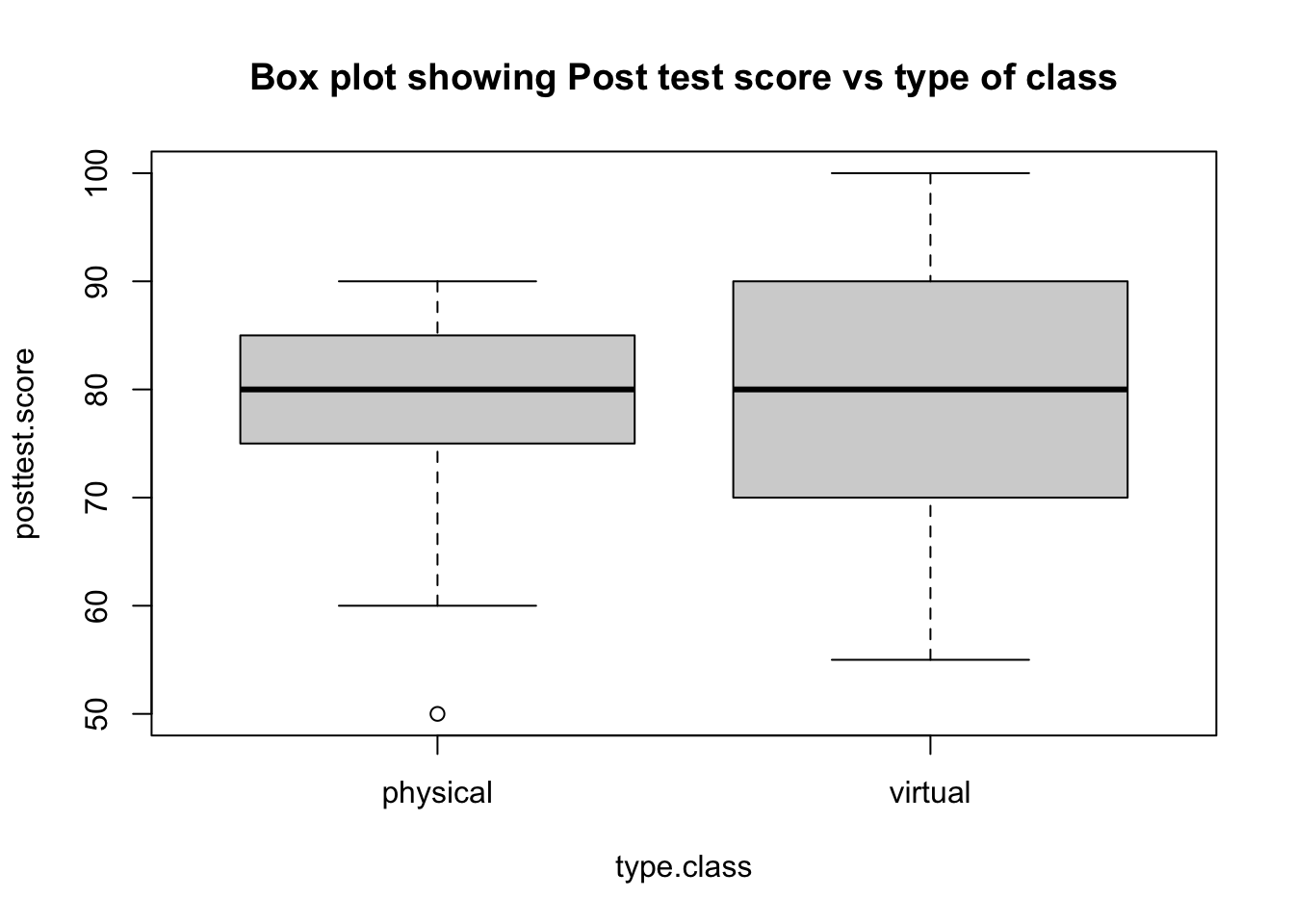
Code
boxplot(pretest.score~type.class,main="Box plot showing Pre test score vs type of class")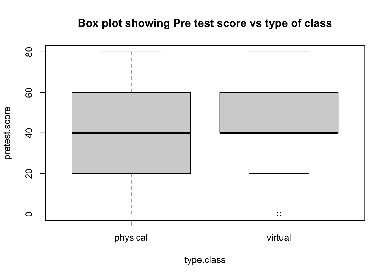
Code
boxplot(total.likert~type.class, main="Box plot showing likert score vs type of class")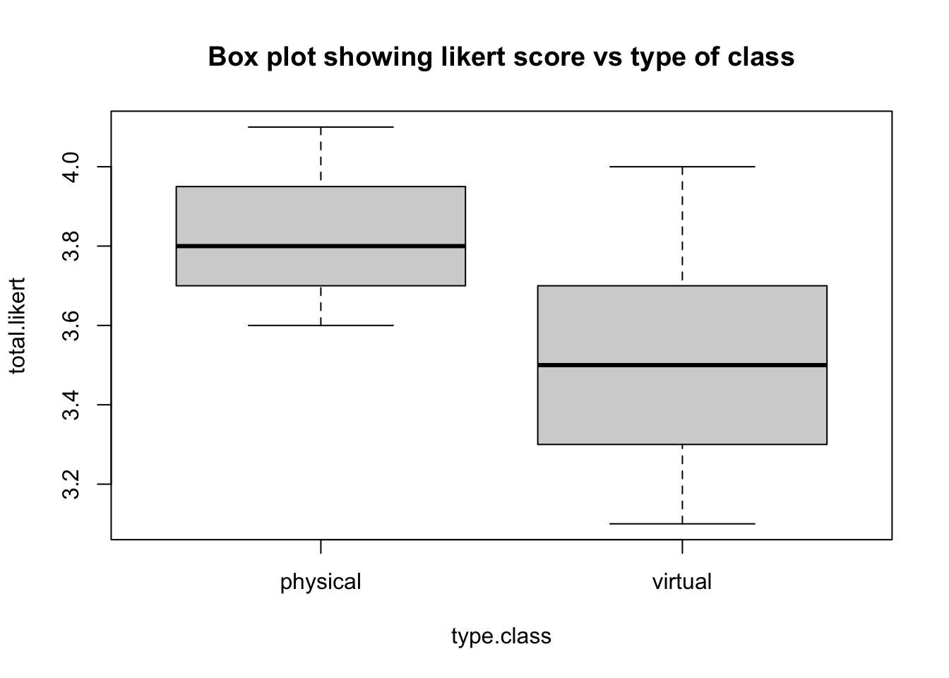
Code
boxplot(total.likert~sex, main="Box plot showing likert score vs sex")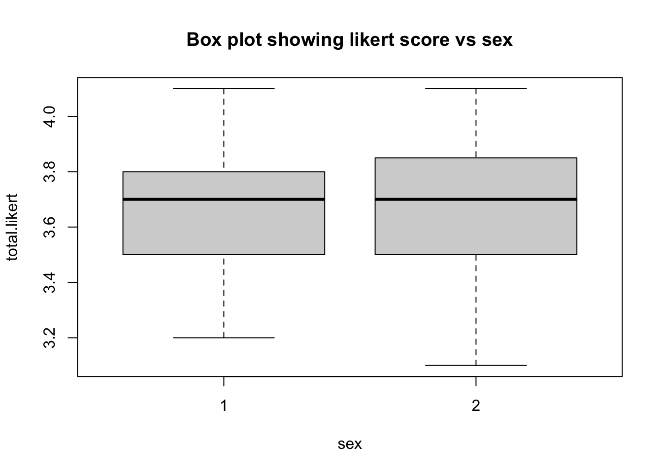
Check for normality visually
hist(posttest.score, main = "",breaks = 15)
hist(total.likert, main="",breaks = 10)
Code
hist(posttest.score, main = "Histogram showing non normal distribution of post test score",breaks = 15)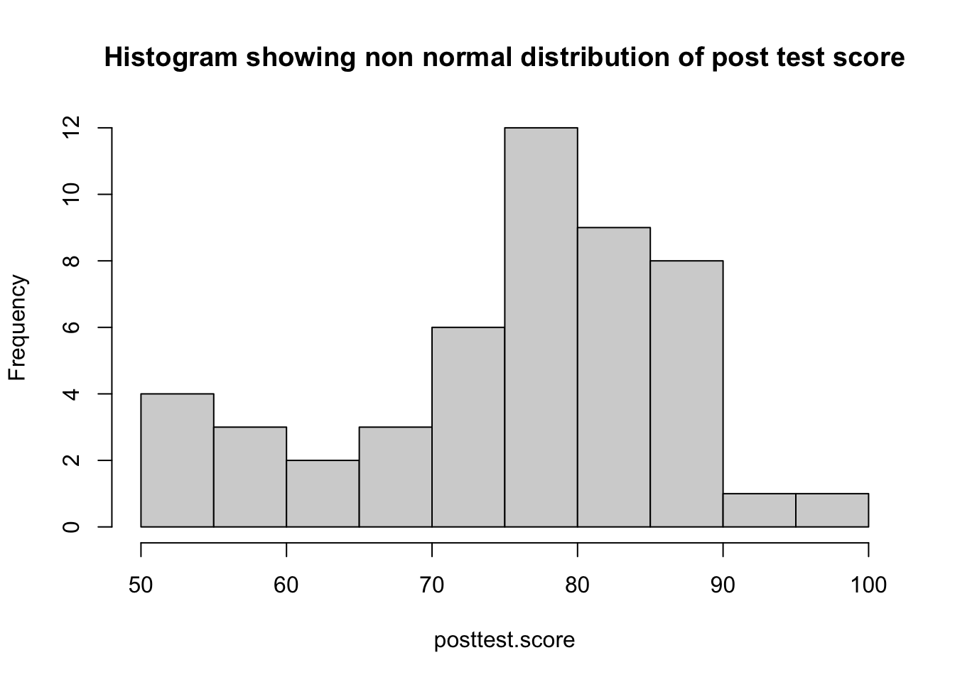
Code
hist(total.likert, main="Histogram showing doubtful normal distribution of likert score",breaks = 10)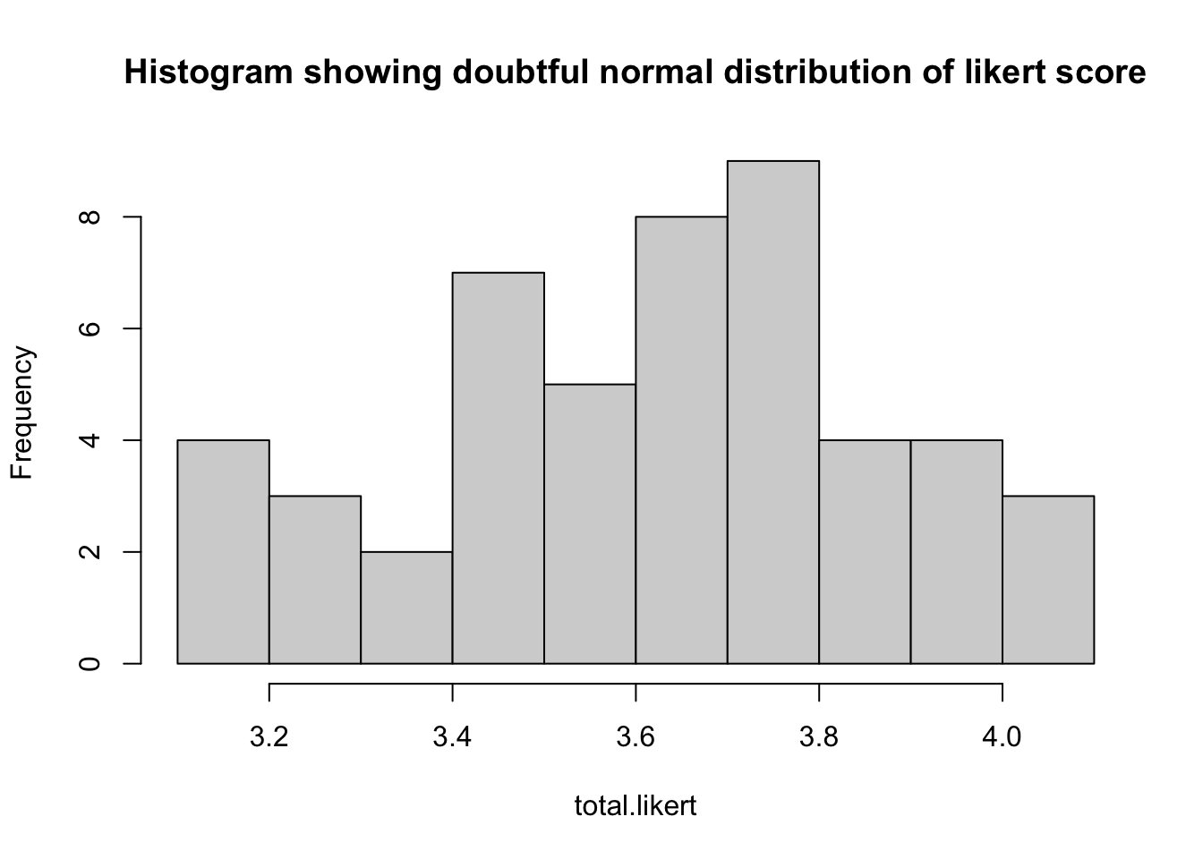
Code
library(ggplot2)
ggplot(fdt)+
  geom_histogram(mapping = aes(x=posttest.score))+
  labs(title = "test")
`stat_bin()` using `bins = 30`. Pick better value with `binwidth`.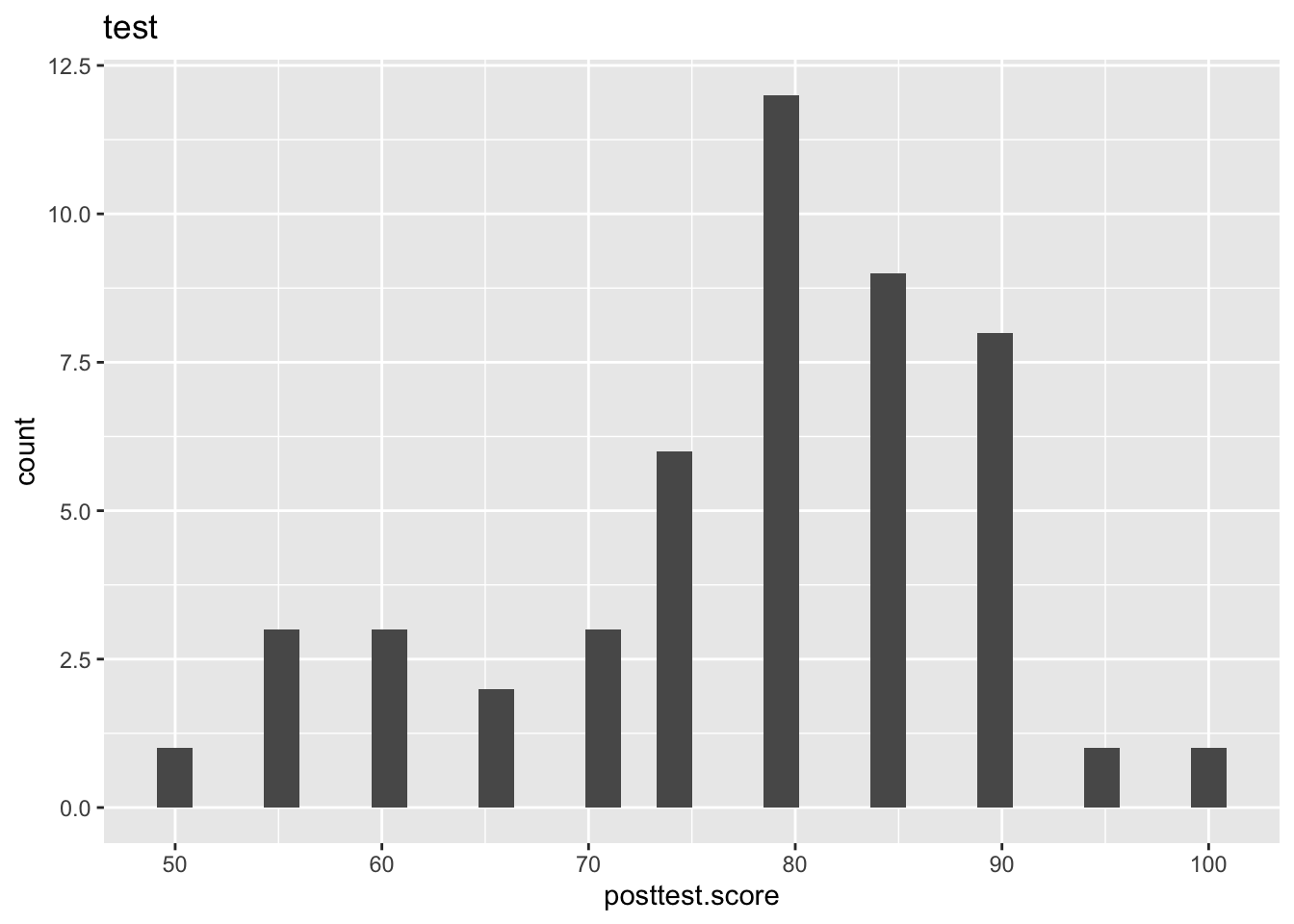
Here we can see that both posttest.score and total.likert are visually not normally distributed. He may cross check it by doing shapiro test
Test for normality
shapiro.test(posttest.score)Code
shapiro.test(posttest.score)
##
##  Shapiro-Wilk normality test
##
## data:  posttest.score
## W = 0.92716, p-value = 0.004812
a p value of <.005 suggest that posttest score is significantly not normal.
Welch t test
As data is not normal, we have to do modified t test.
t.test(posttest.score,pretest.score,var.equal=FALSE)Code
t.test(posttest.score,pretest.score,var.equal=FALSE)
##
##  Welch Two Sample t-test
##
## data:  posttest.score and pretest.score
## t = 10.032, df = 71.146, p-value = 2.929e-15
## alternative hypothesis: true difference in means is not equal to 0
## 95 percent confidence interval:
##  29.18870 43.66845
## sample estimates:
## mean of x mean of y
## 78.06122 41.63265t.test(posttest.score~type.class,var.equal=FALSE)Code
t.test(posttest.score~type.class,var.equal=FALSE)
##
##  Welch Two Sample t-test
##
## data:  posttest.score by type.class
## t = -0.085737, df = 45.72, p-value = 0.932
## alternative hypothesis: true difference in means between group physical and group virtual is not equal to 0
## 95 percent confidence interval:
##  -6.936392  6.369726
## sample estimates:
## mean in group physical  mean in group virtual
##               77.91667               78.20000
Shapiro test for total.likert
shapiro.test(total.likert)Code
shapiro.test(total.likert)
##
##  Shapiro-Wilk normality test
##
## data:  total.likert
## W = 0.96471, p-value = 0.1479
Here the shapiro test is not significant. So the data can be taken as normal.
t.test(total.likert~type.class)Code
t.test(total.likert~type.class)
##
##  Welch Two Sample t-test
##
## data:  total.likert by type.class
## t = 5.9265, df = 42.974, p-value = 4.686e-07
## alternative hypothesis: true difference in means between group physical and group virtual is not equal to 0
## 95 percent confidence interval:
##  0.2172646 0.4414021
## sample estimates:
## mean in group physical  mean in group virtual
##               3.833333               3.504000
Creating breaks
{r}
age=c(1:100)
dtb=data.table(age=age,sex=c(rbinom(n = 100,size = 1,prob = .5)))
dtb$class=cut(dtb$age,breaks = c(0,13,28,60,75,101),labels = c("child","young","mature","old","aged"))
head(dtb)
Code
age=c(1:100)
dtb=data.table(age=age,sex=c(rbinom(n = 100,size = 1,prob = .5)))
dtb$class=cut(dtb$age,breaks = c(0,13,28,60,75,101),labels = c("child","young","mature","old","aged"))
head(dtb)
age sex class
<int> <int> <fctr>
1: 1 0 child
2: 2 1 child
3: 3 0 child
4: 4 1 child
5: 5 0 child
6: 6 1 childMaking data wide
{r}
dtw=dcast(data = dtb,formula = age~sex,value.var = "class")
head(dtw)
Code
dtw=dcast(data = dtb,formula = age~sex,value.var = "class")
head(dtw)
Key: <age>
age 0 1
<int> <fctr> <fctr>
1: 1 child <NA>
2: 2 <NA> child
3: 3 child <NA>
4: 4 <NA> child
5: 5 child <NA>
6: 6 <NA> childFootnotes
Now from r 4.1 onwards it is built in to base v as I >↩︎
note that, [1:2,] is not necessary. However [1:2,] shows the full picture.
↩︎Select first 2 rows and retain all the columns
dt[,.(j)]: blank followed by , denotes selecting all rows. “.” denote “list”. if “
."is not used, data.table will give the output as vectors, instead of list.↩︎The walrus is a large pinniped marine mammal with discontinuous distribution about the North Pole in the Arctic Ocean and subarctic seas of the Northern Hemisphere. ↩︎